SPARK – streaming

The main goal is to make it easier to build end-to-endstreaming applications, which integrate with storage, serving systems, and batch jobs in a consistent and fault-tolerant way


SELECT action, WINDOW(time, “1 hour”), COUNT(*)

FROM events

GROUP BY action, WINDOW(time, “1 hour”)
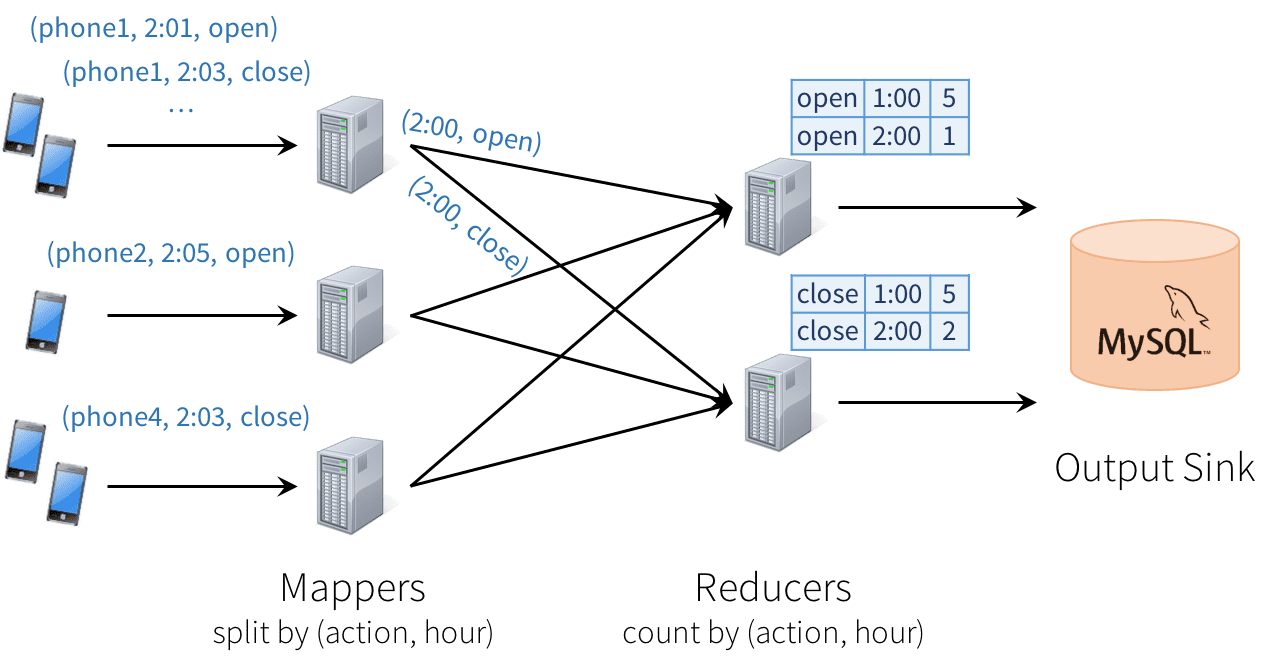
 

image00


Unfortunately, this type of design can introduce quite a few challenges:

  1. Consistency: This distributed design can cause records to be processed in one part of the system before they’re processed in another, leading to nonsensical results. For example, suppose our app sends an “open” event when users open it, and a “close” event when closed. If the reducer node responsible for “open” is slower than the one for “close”, we might see a higher total count of “closes” than “opens” in MySQL, which would not make sense. The image above actually shows one such example.
  2. Fault tolerance: What happens if one of the mappers or reducers fails? A reducer should not count an action in MySQL twice, but should somehow know how to request old data from the mappers when it comes up. Streaming engines go through a great deal of trouble to provide strong semantics here, at least within the engine. In many engines, however, keeping the result consistent in external storage is left to the user.
  3. Out-of-order data: In the real world, data from different sources can come out of order: for example, a phone might upload its data hours late if it’s out of coverage. Just writing the reducer operators to assume data arrives in order of time fields will not work—they need to be prepared to receive out-of-order data, and to update the results in MySQL accordingly.


Structured Streaming Model

In Structured Streaming, we tackle the issue of semantics head-on by making a strong guarantee about the system: at any time, the output of the application is equivalent to executing a batch job on a prefix of the data. For example, in our monitoring application, the result table in MySQL will always be equivalent to taking a prefix of each phone’s update stream (whatever data made it to the system so far) and running the SQL query we showed above. There will never be “open” events counted faster than “close” events, duplicate updates on failure, etc. Structured Streaming automatically handles consistency and reliability both within the engine and in interactions with external systems (e.g. updating MySQL transactionally).

This prefix integrity guarantee makes it easy to reason about the three challenges we identified. In particular:

  1. Output tables are always consistent with all the records in a prefix of the data. For example, as long as each phone uploads its data as a sequential stream (e.g., to the same partition in Apache Kafka), we will always process and count its events in order.
  1. Fault tolerance is handled holistically by Structured Streaming, including in interactions with output sinks. This was a major goal in supporting continuous applications.
  2. The effect of out-of-order data is clear. We know that the job outputs counts grouped by action and time for a prefix of the stream. If we later receive more data, we might see a time field for an hour in the past, and we will simply update its respective row in MySQL.

Users just describe the query they want to run, the input and output locations, and optionally a few more details. The system then runs their query incrementally, maintaining enough state to recover from failure, keep the results consistent in external storage, etc. For example, here is how to write our streaming monitoring application:


  1. // Read data continuously from an S3 location
  2. val inputDF = spark.readStream.json(“s3://logs”)
  3. // Do operations using the standard DataFrame API and write to MySQL
  4. inputDF.groupBy($“action”, window($“time”, “1 hour”)).count()
  5. .writeStream.format(“jdbc”)
  6. .start(“jdbc:mysql//…”)


Model Details

Conceptually, Structured Streaming treats all the data arriving as an unbounded input table. Each new item in the stream is like a row appended to the input table. We won’t actually retain all the input, but our results will be equivalent to having all of it and running a batch job.
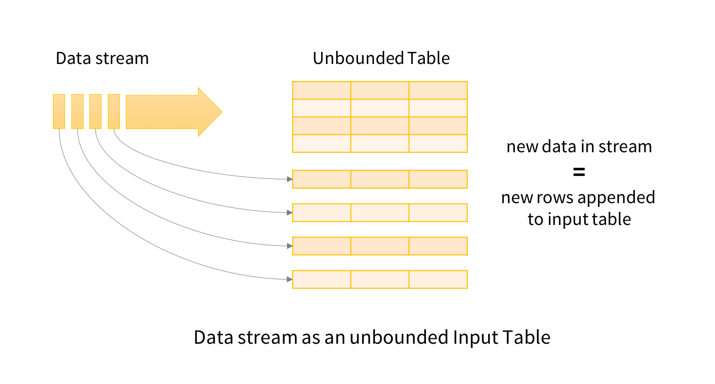
image01

The developer then defines a query on this input table, as if it were a static table, to compute a final result table that will be written to an output sink. Spark automatically converts this batch-like query to a streaming execution plan. This is called incrementalization: Spark figures out what state needs to be maintained to update the result each time a record arrives. Finally, developers specify triggers to control when to update the results. Each time a trigger fires, Spark checks for new data (new row in the input table), and incrementally updates the result.

structured-model

The last part of the model is output modes. Each time the result table is updated, the developer wants to write the changes to an external system, such as S3, HDFS, or a database. We usually want to write output incrementally. For this purpose, Structured Streaming provides three output modes:

  • Append: Only the new rows appended to the result table since the last trigger will be written to the external storage. This is applicable only on queries where existing rows in the result table cannot change (e.g. a map on an input stream).
  • Complete: The entire updated result table will be written to external storage.
  • Update: Only the rows that were updated in the result table since the last trigger will be changed in the external storage. This mode works for output sinks that can be updated in place, such as a MySQL table.


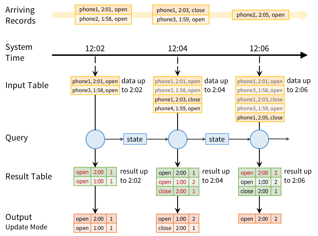
To run this query incrementally, Spark will maintain some state with the counts for each pair so far, and update when new records arrive. For each record changed, it will then output data according to its output mode. The figure below shows this execution using the Update output mode:

stream-example


However, the prefix integrity guarantee in Structured Streaming ensures that we process the records from each source in the order they arrive. For example, because phone1’s “close” event arrives after its “open” event, we will always update the “open” count before we update the “close” count.

Fault Recovery and Storage System Requirements

Structured Streaming keeps its results valid even if machines fail. To do this, it places two requirements on the input sources and output sinks:

  1. Input sources must be replayable, so that recent data can be re-read if the job crashes. For example, message buses like Amazon Kinesis and Apache Kafka are replayable, as is the file system input source. Only a few minutes’ worth of data needs to be retained; Structured Streaming will maintain its own internal state after that.
  2. Output sinks must support transactional updates, so that the system can make a set of records appear atomically. The current version of Structured Streaming implements this for file sinks, and we also plan to add it for common databases and key-value stores.

We found that most Spark applications already use sinks and sources with these properties, because users want their jobs to be reliable.

Apart from these requirements, Structured Streaming will manage its internal state in a reliable storage system, such as S3 or HDFS, to store data such as the running counts in our example. Given these properties, Structured Streaming will enforce prefix integrity end-to-end.

It also adds new operators for windowed aggregation and for setting parameters of the execution model (e.g. output modes). In Apache Spark 2.0, we’ve built an alpha version of the system with the core APIs. More operators, such as sessionization, will come in future releases.


Streams in Structured Streaming are represented as DataFrames or Datasets with the isStreaming property set to true

  1. val inputDF = spark.readStream.json(“s3://logs”)
  1. val countsDF = inputDF.groupBy($“action”, window($“time”, “1 hour”))
  2. .count()

The new DataFrame countsDF is our result table, which has the columns action, window, and count, and will be continuously updated when the query is started. Note that this transformation would give hourly counts even if inputDF was a static table. This allows developers to test their business logic on static datasets and seamless apply them on streaming data without changing the logic.

Finally, we tell the engine to write this table to a sink and start the streaming computation.

  1. val query = countsDF.writeStream.format(“jdbc”).start(“jdbc://…”)


The returned query is a StreamingQuery, a handle to the active streaming execution and can be used to manage and monitor the execution.


Windowed Aggregations on Event Time

Streaming applications often need to compute data on various types of windows, including sliding windows, which overlap with each other (e.g. a 1-hour window that advances every 5 minutes), and tumbling windows, which do not (e.g. just every hour). In Structured Streaming, windowing is simply represented as a group-by. Each input event can be mapped to one or more windows, and simply results in updating one or more result table rows.

Windows can be specified using the window function in DataFrames. For example, we could change our monitoring job to count actions by sliding windows as follows:

  1. inputDF.groupBy($“action”, window($“time”, “1 hour”, “5 minutes”))
  2. .count()

Whereas our previous application outputted results of the form (hour, action, count), this new one will output results of the form (window, action, count), such as (“1:10-2:10”, “open”, 17). If a late record arrives, we will update all the corresponding windows in MySQL. And unlike in many other systems, windowing is not just a special operator for streaming computations; we can run the same code in a batch job to group data in the same way.


Windowed aggregation is one area where we will continue to expand Structured Streaming. In particular, in Spark 2.1, we plan to add watermarks, a feature for dropping overly old data when sufficient time has passed. Without this type of feature, the system might have to track state for all old windows, which would not scale as the application runs. In addition, we plan to add support for session-based windows, i.e. grouping the events from one source into variable-length sessions according to business logic.

Joining Streams with Static Data

Because Structured Streaming simply uses the DataFrame API, it is straightforward to join a stream against a static DataFrame, such as an Apache Hive table:

  1. // Bring in data about each customer from a static “customers” table,
  2. // then join it with a streaming DataFrame
  3. val customersDF = spark.table(“customers”)
  4. inputDF.join(customersDF, “customer_id”)
  5. .groupBy($“customer_name”, hour($“time”))
  6. .count()

Interactive Queries

Structured Streaming can expose results directly to interactive queries through Spark’s JDBC server. In Spark 2.0, there is a rudimentary “memory” output sink for this purpose that is not designed for large data volumes. However, in future releases, this will let you write query results to an in-memory Spark SQL table, and run queries directly against it.

  1. // Save our previous counts query to an in-memory table
  2. countsDF.writeStream.format(“memory”)
  3. .queryName(“counts”)
  4. .outputMode(“complete”)
  5. .start()
  6.  
  7. // Then any thread can query the table using SQL
  8. sql(“select sum(count) from counts where action=’login'”)


spark – partition

By default, a partition is created for each HDFS partition, which by default is 64MB (from Spark’s Programming Guide).

RDDs get partitioned automatically without programmer intervention. However, there are times when you’d like to adjust the size and number of partitions or the partitioning scheme according to the needs of your application.

You use def getPartitions: Array[Partition] method on a RDD to know the set of partitions in this RDD.

When a stage executes, you can see the number of partitions for a given stage in the Spark UI

The reason for 8 Tasks in Total is that I’m on a 8-core laptop and by default the number of partitions is the number of all available cores.

You can request for the minimum number of partitions, using the second input parameter to many transformations.

Spark can only run 1 concurrent task for every partition of an RDD, up to the number of cores in your cluster. So if you have a cluster with 50 cores, you want your RDDs to at least have 50 partitions (and probably 2-3x times that).

As far as choosing a “good” number of partitions, you generally want at least as many as the number of executors for parallelism. You can get this computed value by calling sc.defaultParallelism.

Also, the number of partitions determines how many files get generated by actions that save RDDs to files.

The maximum size of a partition is ultimately limited by the available memory of an executor.

In the first RDD transformation, e.g. reading from a file using sc.textFile(path, partition), the partition parameter will be applied to all further transformations and actions on this RDD.

Partitions get redistributed among nodes whenever shuffle occurs. Repartitioning may cause shuffleto occur in some situations, but it is not guaranteed to occur in all cases. And it usually happens during action stage.

When creating an RDD by reading a file using rdd = SparkContext().textFile("hdfs://…/file.txt") the number of partitions may be smaller. Ideally, you would get the same number of blocks as you see in HDFS, but if the lines in your file are too long (longer than the block size), there will be fewer partitions.

Preferred way to set up the number of partitions for an RDD is to directly pass it as the second input parameter in the call like rdd = sc.textFile("hdfs://…/file.txt", 400), where 400 is the number of partitions. In this case, the partitioning makes for 400 splits that would be done by the Hadoop’s TextInputFormat, not Spark and it would work much faster. It’s also that the code spawns 400 concurrent tasks to try to load file.txt directly into 400 partitions.

It will only work as described for uncompressed files.

When using textFile with compressed files (file.txt.gz not file.txt or similar), Spark disables splitting that makes for an RDD with only 1 partition (as reads against gzipped files cannot be parallelized). In this case, to change the number of partitions you should do repartitioning.

2

Some operations, e.g. map, flatMap, filter, don’t preserve partitioning.

3

map, flatMap, filter operations apply a function to every partition.

Repartitioning RDD — repartition Transformation

repartition(numPartitions: Int)(implicit ord: Ordering[T] = null): RDD[T]

repartition is coalesce with numPartitions and shuffle enabled.

With the following computation you can see that repartition(5) causes 5 tasks to be started using NODE_LOCALdata locality.

Please note that Spark disables splitting for compressed files and creates RDDs with only 1 partition. In such cases, it’s helpful to use sc.textFile('demo.gz') and do repartitioning using rdd.repartition(100) as follows:

rdd = sc.textFile('demo.gz')
rdd = rdd.repartition(100)

With the lines, you end up with rdd to be exactly 100 partitions of roughly equal in size.

  • rdd.repartition(N) does a shuffle to split data to match N

    • partitioning is done on round robin basis

    Please note that Spark disables splitting for compressed files and creates RDDs with only 1 partition. In such cases, it’s helpful to use sc.textFile('demo.gz') and do repartitioning using rdd.repartition(100) as follows:

    rdd = sc.textFile('demo.gz')
    rdd = rdd.repartition(100)

    With the lines, you end up with rdd to be exactly 100 partitions of roughly equal in size.

    • rdd.repartition(N) does a shuffle to split data to match N

      • partitioning is done on round robin basis


spark – performance

Data Locality

Data locality can have a major impact on the performance of Spark jobs. If data and the code that operates on it are together then computation tends to be fast. But if code and data are separated, one must move to the other. Typically it is faster to ship serialized code from place to place than a chunk of data because code size is much smaller than data. Spark builds its scheduling around this general principle of data locality.

Data locality is how close data is to the code processing it. There are several levels of locality based on the data’s current location. In order from closest to farthest:

  • PROCESS_LOCAL data is in the same JVM as the running code. This is the best locality possible
  • NODE_LOCAL data is on the same node. Examples might be in HDFS on the same node, or in another executor on the same node. This is a little slower than PROCESS_LOCAL because the data has to travel between processes
  • NO_PREF data is accessed equally quickly from anywhere and has no locality preference
  • RACK_LOCAL data is on the same rack of servers. Data is on a different server on the same rack so needs to be sent over the network, typically through a single switch
  • ANY data is elsewhere on the network and not in the same rack

Spark prefers to schedule all tasks at the best locality level, but this is not always possible. In situations where there is no unprocessed data on any idle executor, Spark switches to lower locality levels. There are two options: a) wait until a busy CPU frees up to start a task on data on the same server, or b) immediately start a new task in a farther away place that requires moving data there.

What Spark typically does is wait a bit in the hopes that a busy CPU frees up. Once that timeout expires, it starts moving the data from far away to the free CPU. The wait timeout for fallback between each level can be configured individually or all together in one parameter; see thespark.locality parameters on the configuration page for details. You should increase these settings if your tasks are long and see poor locality, but the default usually works well.

spark – actions

Actions

The following table lists some of the common actions supported by Spark. Refer to the RDD API doc (Scala, Java, Python, R)

and pair RDD functions doc (Scala, Java) for details.

Action Meaning
reduce(func) Aggregate the elements of the dataset using a function func (which takes two arguments and returns one). The function should be commutative and associative so that it can be computed correctly in parallel.
collect() Return all the elements of the dataset as an array at the driver program. This is usually useful after a filter or other operation that returns a sufficiently small subset of the data.
count() Return the number of elements in the dataset.
first() Return the first element of the dataset (similar to take(1)).
take(n) Return an array with the first n elements of the dataset.
takeSample(withReplacement, num, [seed]) Return an array with a random sample of num elements of the dataset, with or without replacement, optionally pre-specifying a random number generator seed.
takeOrdered(n, [ordering]) Return the first n elements of the RDD using either their natural order or a custom comparator.
saveAsTextFile(path) Write the elements of the dataset as a text file (or set of text files) in a given directory in the local filesystem, HDFS or any other Hadoop-supported file system. Spark will call toString on each element to convert it to a line of text in the file.
saveAsSequenceFile(path)
(Java and Scala)
Write the elements of the dataset as a Hadoop SequenceFile in a given path in the local filesystem, HDFS or any other Hadoop-supported file system. This is available on RDDs of key-value pairs that implement Hadoop’s Writable interface. In Scala, it is also available on types that are implicitly convertible to Writable (Spark includes conversions for basic types like Int, Double, String, etc).
saveAsObjectFile(path)
(Java and Scala)
Write the elements of the dataset in a simple format using Java serialization, which can then be loaded using SparkContext.objectFile().
countByKey() Only available on RDDs of type (K, V). Returns a hashmap of (K, Int) pairs with the count of each key.
foreach(func) Run a function func on each element of the dataset. This is usually done for side effects such as updating an Accumulator or interacting with external storage systems.
Note: modifying variables other than Accumulators outside of the foreach() may result in undefined behavior. See Understanding closures for more details.

The Spark RDD API also exposes asynchronous versions of some actions, like foreachAsync for foreach, which immediately return a FutureAction to the caller instead of blocking on completion of the action. This can be used to manage or wait for the asynchronous execution of the action.

spark – transformations

https://spark.apache.org/docs/latest/api/scala/index.html#org.apache.spark.rdd.RDD

https://spark.apache.org/docs/latest/api/scala/index.html#org.apache.spark.rdd.PairRDDFunctions

flatMap(func) Similar to map, but each input item can be mapped to 0 or more output items (so funcshould return a Seq rather than a single item).
mapPartitions(func) Similar to map, but runs separately on each partition (block) of the RDD, so func must be of type Iterator<T> => Iterator<U> when running on an RDD of type T.
mapPartitionsWithIndex(func) Similar to mapPartitions, but also provides func with an integer value representing the index of the partition, so func must be of type (Int, Iterator<T>) => Iterator<U> when running on an RDD of type T.
sample(withReplacement, fraction, seed) Sample a fraction fraction of the data, with or without replacement, using a given random number generator seed.


groupByKey([numTasks]) When called on a dataset of (K, V) pairs, returns a dataset of (K, Iterable<V>) pairs.
Note: If you are grouping in order to perform an aggregation (such as a sum or average) over each key, using reduceByKey or aggregateByKey will yield much better performance.
Note: By default, the level of parallelism in the output depends on the number of partitions of the parent RDD. You can pass an optional numTasks argument to set a different number of tasks.


reduceByKey(func, [numTasks]) When called on a dataset of (K, V) pairs, returns a dataset of (K, V) pairs where the values for each key are aggregated using the given reduce function func, which must be of type (V,V) => V. Like in groupByKey, the number of reduce tasks is configurable through an optional second argument.
aggregateByKey(zeroValue)(seqOp, combOp, [numTasks]) When called on a dataset of (K, V) pairs, returns a dataset of (K, U) pairs where the values for each key are aggregated using the given combine functions and a neutral “zero” value. Allows an aggregated value type that is different than the input value type, while avoiding unnecessary allocations. Like in groupByKey, the number of reduce tasks is configurable through an optional second argument.
sortByKey([ascending], [numTasks]) When called on a dataset of (K, V) pairs where K implements Ordered, returns a dataset of (K, V) pairs sorted by keys in ascending or descending order, as specified in the boolean ascending argument.
join(otherDataset, [numTasks]) When called on datasets of type (K, V) and (K, W), returns a dataset of (K, (V, W)) pairs with all pairs of elements for each key. Outer joins are supported through leftOuterJoin, rightOuterJoin, and fullOuterJoin.
cogroup(otherDataset, [numTasks]) When called on datasets of type (K, V) and (K, W), returns a dataset of (K, (Iterable<V>, Iterable<W>)) tuples. This operation is also called groupWith.
cartesian(otherDataset) When called on datasets of types T and U, returns a dataset of (T, U) pairs (all pairs of elements).
pipe(command, [envVars]) Pipe each partition of the RDD through a shell command, e.g. a Perl or bash script. RDD elements are written to the process’s stdin and lines output to its stdout are returned as an RDD of strings.
coalesce(numPartitions) Decrease the number of partitions in the RDD to numPartitions. Useful for running operations more efficiently after filtering down a large dataset.
repartition(numPartitions) Reshuffle the data in the RDD randomly to create either more or fewer partitions and balance it across them. This always shuffles all data over the network.
repartitionAndSortWithinPartitions(partitioner) Repartition the RDD according to the given partitioner and, within each resulting partition, sort records by their keys. This is more efficient than calling repartition and then sorting within each partition because it can push the sorting down into the shuffle machinery.


spark – architecture , basics

Diving into Apache Spark: Part 3

http://blog.cloudera.com/blog/2015/03/how-to-tune-your-apache-spark-jobs-part-1/

https://0x0fff.com/spark-architecture/#comments

http://homepage.cs.latrobe.edu.au/zhe/ZhenHeSparkRDDAPIExamples.html#keyBy

kafka – use cases

1.2 Use Cases

Here is a description of a few of the popular use cases for Apache Kafka™. For an overview of a number of these areas in action, see this blog post.

Messaging

Kafka works well as a replacement for a more traditional message broker. Message brokers are used for a variety of reasons (to decouple processing from data producers, to buffer unprocessed messages, etc). In comparison to most messaging systems Kafka has better throughput, built-in partitioning, replication, and fault-tolerance which makes it a good solution for large scale message processing applications.

In our experience messaging uses are often comparatively low-throughput, but may require low end-to-end latency and often depend on the strong durability guarantees Kafka provides.

In this domain Kafka is comparable to traditional messaging systems such as ActiveMQ or RabbitMQ.

Website Activity Tracking

The original use case for Kafka was to be able to rebuild a user activity tracking pipeline as a set of real-time publish-subscribe feeds. This means site activity (page views, searches, or other actions users may take) is published to central topics with one topic per activity type. These feeds are available for subscription for a range of use cases including real-time processing, real-time monitoring, and loading into Hadoop or offline data warehousing systems for offline processing and reporting.

Activity tracking is often very high volume as many activity messages are generated for each user page view.

Metrics

Kafka is often used for operational monitoring data. This involves aggregating statistics from distributed applications to produce centralized feeds of operational data.

Log Aggregation

Many people use Kafka as a replacement for a log aggregation solution. Log aggregation typically collects physical log files off servers and puts them in a central place (a file server or HDFS perhaps) for processing. Kafka abstracts away the details of files and gives a cleaner abstraction of log or event data as a stream of messages. This allows for lower-latency processing and easier support for multiple data sources and distributed data consumption. In comparison to log-centric systems like Scribe or Flume, Kafka offers equally good performance, stronger durability guarantees due to replication, and much lower end-to-end latency.

Stream Processing

Many users of Kafka process data in processing pipelines consisting of multiple stages, where raw input data is consumed from Kafka topics and then aggregated, enriched, or otherwise transformed into new topics for further consumption or follow-up processing. For example, a processing pipeline for recommending news articles might crawl article content from RSS feeds and publish it to an “articles” topic; further processing might normalize or deduplicate this content and published the cleansed article content to a new topic; a final processing stage might attempt to recommend this content to users. Such processing pipelines create graphs of real-time data flows based on the individual topics. Starting in 0.10.0.0, a light-weight but powerful stream processing library called Kafka Streams is available in Apache Kafka to perform such data processing as described above. Apart from Kafka Streams, alternative open source stream processing tools include Apache Storm and Apache Samza.

Event Sourcing

Event sourcing is a style of application design where state changes are logged as a time-ordered sequence of records. Kafka’s support for very large stored log data makes it an excellent backend for an application built in this style.

Commit Log

Kafka can serve as a kind of external commit-log for a distributed system. The log helps replicate data between nodes and acts as a re-syncing mechanism for failed nodes to restore their data. The log compaction feature in Kafka helps support this usage. In this usage Kafka is similar to Apache BookKeeper project.

cassandra – consistency level – default ‘ONE’

Configuring client consistency levels 

You can use a new cqlsh command, CONSISTENCY, to set the consistency level for queries from the current cqlsh session. The WITH CONSISTENCY clause has been removed from CQL commands. You set the consistency level programmatically (at the driver level). For example, call QueryBuilder.insertInto with a setConsistencyLevel argument. The consistency level defaults to ONE for all write and read operations.

cassandra – read consistency

About read consistency 

The consistency level specifies how many replicas must respond to a read request before returning data to the client application.

Cassandra checks the specified number of replicas for data to satisfy the read request.

Read Consistency Levels
Level Description Usage
ALL Returns the record after all replicas have responded. The read operation will fail if a replica does not respond. Provides the highest consistency of all levels and the lowest availability of all levels.
EACH_QUORUM Not supported for reads. Not supported for reads.
QUORUM Returns the record after a quorum of replicas has responded from any data center. Ensures strong consistency if you can tolerate some level of failure.
LOCAL_QUORUM Returns the record after a quorum of replicas in the current data center as the coordinator has reported. Avoids latency of inter-data center communication. Used in multiple data center clusters with a rack-aware replica placement strategy ( NetworkTopologyStrategy) and a properly configured snitch. Fails when using SimpleStrategy.
ONE Returns a response from the closest replica, as determined by the snitch. By default, a read repair runs in the background to make the other replicas consistent. Provides the highest availability of all the levels if you can tolerate a comparatively high probability of stale data being read. The replicas contacted for reads may not always have the most recent write.
TWO Returns the most recent data from two of the closest replicas. Similar to ONE.
THREE Returns the most recent data from three of the closest replicas. Similar to TWO.
LOCAL_ONE Returns a response from the closest replica in the local data center. Same usage as described in the table about write consistency levels.
SERIAL Allows reading the current (and possibly uncommitted) state of data without proposing a new addition or update. If a SERIAL read finds an uncommitted transaction in progress, it will commit the transaction as part of the read. Similar to QUORUM. To read the latest value of a column after a user has invoked a lightweight transaction to write to the column, use SERIAL. Cassandra then checks the inflight lightweight transaction for updates and, if found, returns the latest data.
LOCAL_SERIAL Same as SERIAL, but confined to the data center. Similar to LOCAL_QUORUM. Used to achieve linearizable consistency for lightweight transactions.

cassandra – write consistency

The consistency level determines the number of replicas on which the write must succeed before returning an acknowledgment to the client application.

Write Consistency Levels
Level Description Usage
ALL A write must be written to the commit log and memtable on all replica nodes in the cluster for that partition key. Provides the highest consistency and the lowest availability of any other level.
EACH_QUORUM Strong consistency. A write must be written to the commit log and memtable on a quorum of replica nodes in all data center. Used in multiple data center clusters to strictly maintain consistency at the same level in each data center. For example, choose this level if you want a read to fail when a data center is down and the QUORUM cannot be reached on that data center.
QUORUM A write must be written to the commit log and memtable on a quorum of replica nodes.

Provides strong consistency if you can tolerate some level of failure.

LOCAL_QUORUM Strong consistency. A write must be written to the commit log and memtable on a quorum of replica nodes in the same data center as thecoordinator node. Avoids latency of inter-data center communication. Used in multiple data center clusters with a rack-aware replica placement strategy, such as NetworkTopologyStrategy, and a properly configured snitch. Use to maintain consistency locally (within the single data center). Can be used with SimpleStrategy.
ONE A write must be written to the commit log and memtable of at least one replica node. Satisfies the needs of most users because consistency requirements are not stringent.
TWO A write must be written to the commit log and memtable of at least two replica nodes. Similar to ONE.
THREE A write must be written to the commit log and memtable of at least three replica nodes. Similar to TWO.
LOCAL_ONE A write must be sent to, and successfully acknowledged by, at least one replica node in the local data center. In a multiple data center clusters, a consistency level of ONE is often desirable, but cross-DC traffic is not. LOCAL_ONE accomplishes this. For security and quality reasons, you can use this consistency level in an offline datacenter to prevent automatic connection to online nodes in other data centers if an offline node goes down.
ANY A write must be written to at least one node. If all replica nodes for the given partition key are down, the write can still succeed after a hinted handoff has been written. If all replica nodes are down at write time, an ANY write is not readable until the replica nodes for that partition have recovered. Provides low latency and a guarantee that a write never fails. Delivers the lowest consistency and highest availability.
SERIAL Achieves linearizable consistency for lightweight transactions by preventing unconditional updates. You cannot configure this level as a normal consistency level, configured at the driver level using the consistency level field. You configure this level using the serial consistency field as part of the native protocol operation. See failure scenarios.
LOCAL_SERIAL Same as SERIAL but confined to the data center. A write must be written conditionally to the commit log and memtable on a quorum of replica nodes in the same data center. Same as SERIAL. Used for disaster recovery. See failure scenarios.

Even at low consistency levels, the write is still sent to all replicas for the written key, even replicas in other data centers. The consistency level just determines how many replicas are required to respond that they received the write.