SPARK – streaming

November 30, 2016November 30, 2016 corerootz - Ravi Kiran Krovvidi Spark spark streaming

The main goal is to make it easier to build end-to-endstreaming applications, which integrate with storage, serving systems, and batch jobs in a consistent and fault-tolerant way

SELECT action, WINDOW(time, “1 hour”), COUNT(*)

FROM events

GROUP BY action, WINDOW(time, “1 hour”)

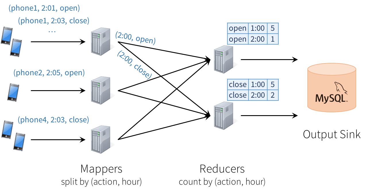
Unfortunately, this type of design can introduce quite a few challenges:

Consistency: This distributed design can cause records to be processed in one part of the system before they’re processed in another, leading to nonsensical results. For example, suppose our app sends an “open” event when users open it, and a “close” event when closed. If the reducer node responsible for “open” is slower than the one for “close”, we might see a higher total count of “closes” than “opens” in MySQL, which would not make sense. The image above actually shows one such example.
Fault tolerance: What happens if one of the mappers or reducers fails? A reducer should not count an action in MySQL twice, but should somehow know how to request old data from the mappers when it comes up. Streaming engines go through a great deal of trouble to provide strong semantics here, at least within the engine. In many engines, however, keeping the result consistent in external storage is left to the user.
Out-of-order data: In the real world, data from different sources can come out of order: for example, a phone might upload its data hours late if it’s out of coverage. Just writing the reducer operators to assume data arrives in order of time fields will not work—they need to be prepared to receive out-of-order data, and to update the results in MySQL accordingly.

Structured Streaming Model

In Structured Streaming, we tackle the issue of semantics head-on by making a strong guarantee about the system: at any time, the output of the application is equivalent to executing a batch job on a prefix of the data. For example, in our monitoring application, the result table in MySQL will always be equivalent to taking a prefix of each phone’s update stream (whatever data made it to the system so far) and running the SQL query we showed above. There will never be “open” events counted faster than “close” events, duplicate updates on failure, etc. Structured Streaming automatically handles consistency and reliability both within the engine and in interactions with external systems (e.g. updating MySQL transactionally).

This prefix integrity guarantee makes it easy to reason about the three challenges we identified. In particular:

Output tables are always consistent with all the records in a prefix of the data. For example, as long as each phone uploads its data as a sequential stream (e.g., to the same partition in Apache Kafka), we will always process and count its events in order.

Fault tolerance is handled holistically by Structured Streaming, including in interactions with output sinks. This was a major goal in supporting continuous applications.
The effect of out-of-order data is clear. We know that the job outputs counts grouped by action and time for a prefix of the stream. If we later receive more data, we might see a time field for an hour in the past, and we will simply update its respective row in MySQL.

Users just describe the query they want to run, the input and output locations, and optionally a few more details. The system then runs their query incrementally, maintaining enough state to recover from failure, keep the results consistent in external storage, etc. For example, here is how to write our streaming monitoring application:

// Read data continuously from an S3 location
val inputDF = spark.readStream.json(“s3://logs”)
// Do operations using the standard DataFrame API and write to MySQL
inputDF.groupBy($“action”, window($“time”, “1 hour”)).count()
.writeStream.format(“jdbc”)
.start(“jdbc:mysql//…”)

Model Details

Conceptually, Structured Streaming treats all the data arriving as an unbounded input table. Each new item in the stream is like a row appended to the input table. We won’t actually retain all the input, but our results will be equivalent to having all of it and running a batch job.

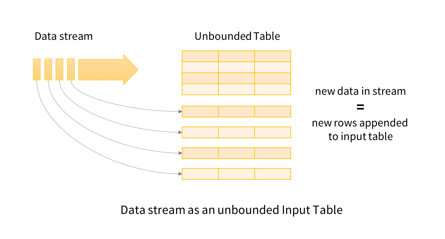
The developer then defines a query on this input table, as if it were a static table, to compute a final result table that will be written to an output sink. Spark automatically converts this batch-like query to a streaming execution plan. This is called incrementalization: Spark figures out what state needs to be maintained to update the result each time a record arrives. Finally, developers specify triggers to control when to update the results. Each time a trigger fires, Spark checks for new data (new row in the input table), and incrementally updates the result.

The last part of the model is output modes. Each time the result table is updated, the developer wants to write the changes to an external system, such as S3, HDFS, or a database. We usually want to write output incrementally. For this purpose, Structured Streaming provides three output modes:

Append: Only the new rows appended to the result table since the last trigger will be written to the external storage. This is applicable only on queries where existing rows in the result table cannot change (e.g. a map on an input stream).
Complete: The entire updated result table will be written to external storage.
Update: Only the rows that were updated in the result table since the last trigger will be changed in the external storage. This mode works for output sinks that can be updated in place, such as a MySQL table.

To run this query incrementally, Spark will maintain some state with the counts for each pair so far, and update when new records arrive. For each record changed, it will then output data according to its output mode. The figure below shows this execution using the Update output mode:

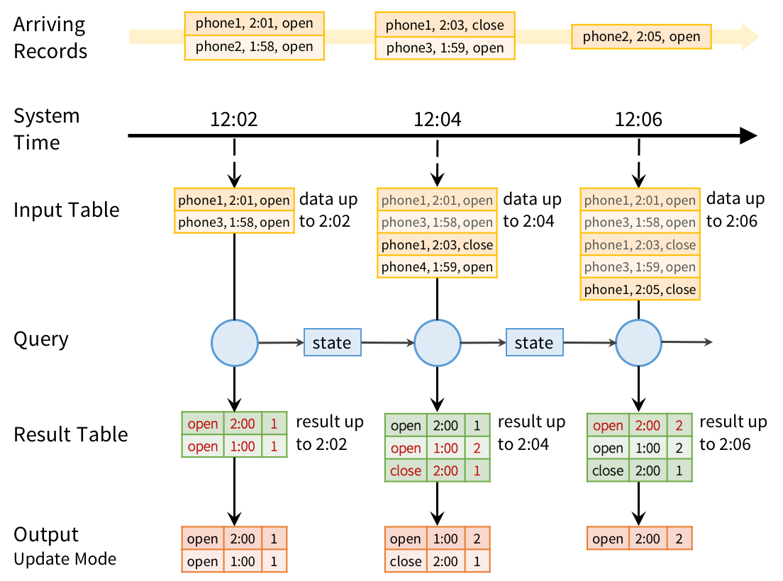
However, the prefix integrity guarantee in Structured Streaming ensures that we process the records from each source in the order they arrive. For example, because phone1’s “close” event arrives after its “open” event, we will always update the “open” count before we update the “close” count.

Fault Recovery and Storage System Requirements

Structured Streaming keeps its results valid even if machines fail. To do this, it places two requirements on the input sources and output sinks:

Input sources must be replayable, so that recent data can be re-read if the job crashes. For example, message buses like Amazon Kinesis and Apache Kafka are replayable, as is the file system input source. Only a few minutes’ worth of data needs to be retained; Structured Streaming will maintain its own internal state after that.
Output sinks must support transactional updates, so that the system can make a set of records appear atomically. The current version of Structured Streaming implements this for file sinks, and we also plan to add it for common databases and key-value stores.

We found that most Spark applications already use sinks and sources with these properties, because users want their jobs to be reliable.

Apart from these requirements, Structured Streaming will manage its internal state in a reliable storage system, such as S3 or HDFS, to store data such as the running counts in our example. Given these properties, Structured Streaming will enforce prefix integrity end-to-end.

It also adds new operators for windowed aggregation and for setting parameters of the execution model (e.g. output modes). In Apache Spark 2.0, we’ve built an alpha version of the system with the core APIs. More operators, such as sessionization, will come in future releases.

Streams in Structured Streaming are represented as DataFrames or Datasets with the isStreaming property set to true

val inputDF = spark.readStream.json(“s3://logs”)

val countsDF = inputDF.groupBy($“action”, window($“time”, “1 hour”))
.count()

The new DataFrame countsDF is our result table, which has the columns action, window, and count, and will be continuously updated when the query is started. Note that this transformation would give hourly counts even if inputDF was a static table. This allows developers to test their business logic on static datasets and seamless apply them on streaming data without changing the logic.

Finally, we tell the engine to write this table to a sink and start the streaming computation.

val query = countsDF.writeStream.format(“jdbc”).start(“jdbc://…”)

The returned query is a StreamingQuery, a handle to the active streaming execution and can be used to manage and monitor the execution.

Windowed Aggregations on Event Time

Streaming applications often need to compute data on various types of windows, including sliding windows, which overlap with each other (e.g. a 1-hour window that advances every 5 minutes), and tumbling windows, which do not (e.g. just every hour). In Structured Streaming, windowing is simply represented as a group-by. Each input event can be mapped to one or more windows, and simply results in updating one or more result table rows.

Windows can be specified using the window function in DataFrames. For example, we could change our monitoring job to count actions by sliding windows as follows:

inputDF.groupBy($“action”, window($“time”, “1 hour”, “5 minutes”))
.count()

Whereas our previous application outputted results of the form (hour, action, count), this new one will output results of the form (window, action, count), such as (“1:10-2:10”, “open”, 17). If a late record arrives, we will update all the corresponding windows in MySQL. And unlike in many other systems, windowing is not just a special operator for streaming computations; we can run the same code in a batch job to group data in the same way.

Windowed aggregation is one area where we will continue to expand Structured Streaming. In particular, in Spark 2.1, we plan to add watermarks, a feature for dropping overly old data when sufficient time has passed. Without this type of feature, the system might have to track state for all old windows, which would not scale as the application runs. In addition, we plan to add support for session-based windows, i.e. grouping the events from one source into variable-length sessions according to business logic.

Joining Streams with Static Data

Because Structured Streaming simply uses the DataFrame API, it is straightforward to join a stream against a static DataFrame, such as an Apache Hive table:

// Bring in data about each customer from a static “customers” table,
// then join it with a streaming DataFrame
val customersDF = spark.table(“customers”)
inputDF.join(customersDF, “customer_id”)
.groupBy($“customer_name”, hour($“time”))
.count()

Interactive Queries

Structured Streaming can expose results directly to interactive queries through Spark’s JDBC server. In Spark 2.0, there is a rudimentary “memory” output sink for this purpose that is not designed for large data volumes. However, in future releases, this will let you write query results to an in-memory Spark SQL table, and run queries directly against it.

// Save our previous counts query to an in-memory table
countsDF.writeStream.format(“memory”)
.queryName(“counts”)
.outputMode(“complete”)
.start()
// Then any thread can query the table using SQL
sql(“select sum(count) from counts where action=’login'”)

spark – partition

November 28, 2016November 28, 2016 corerootz - Ravi Kiran Krovvidi Spark spark architecture

By default, a partition is created for each HDFS partition, which by default is 64MB (from Spark’s Programming Guide).

RDDs get partitioned automatically without programmer intervention. However, there are times when you’d like to adjust the size and number of partitions or the partitioning scheme according to the needs of your application.

You use def getPartitions: Array[Partition] method on a RDD to know the set of partitions in this RDD.

As noted in View Task Execution Against Partitions Using the UI:

When a stage executes, you can see the number of partitions for a given stage in the Spark UI

The reason for 8 Tasks in Total is that I’m on a 8-core laptop and by default the number of partitions is the number of all available cores.

You can request for the minimum number of partitions, using the second input parameter to many transformations.

Spark can only run 1 concurrent task for every partition of an RDD, up to the number of cores in your cluster. So if you have a cluster with 50 cores, you want your RDDs to at least have 50 partitions (and probably 2-3x times that).

As far as choosing a “good” number of partitions, you generally want at least as many as the number of executors for parallelism. You can get this computed value by calling sc.defaultParallelism.

Also, the number of partitions determines how many files get generated by actions that save RDDs to files.

The maximum size of a partition is ultimately limited by the available memory of an executor.

In the first RDD transformation, e.g. reading from a file using sc.textFile(path, partition), the partition parameter will be applied to all further transformations and actions on this RDD.

Partitions get redistributed among nodes whenever shuffle occurs. Repartitioning may cause shuffleto occur in some situations, but it is not guaranteed to occur in all cases. And it usually happens during action stage.

When creating an RDD by reading a file using rdd = SparkContext().textFile("hdfs://…/file.txt") the number of partitions may be smaller. Ideally, you would get the same number of blocks as you see in HDFS, but if the lines in your file are too long (longer than the block size), there will be fewer partitions.

Preferred way to set up the number of partitions for an RDD is to directly pass it as the second input parameter in the call like rdd = sc.textFile("hdfs://…/file.txt", 400), where 400 is the number of partitions. In this case, the partitioning makes for 400 splits that would be done by the Hadoop’s TextInputFormat, not Spark and it would work much faster. It’s also that the code spawns 400 concurrent tasks to try to load file.txt directly into 400 partitions.

It will only work as described for uncompressed files.

When using textFile with compressed files (file.txt.gz not file.txt or similar), Spark disables splitting that makes for an RDD with only 1 partition (as reads against gzipped files cannot be parallelized). In this case, to change the number of partitions you should do repartitioning.

Some operations, e.g. map, flatMap, filter, don’t preserve partitioning.

map, flatMap, filter operations apply a function to every partition.

Repartitioning RDD — `repartition` Transformation

repartition(numPartitions: Int)(implicit ord: Ordering[T] = null): RDD[T]

repartition is coalesce with numPartitions and shuffle enabled.

With the following computation you can see that repartition(5) causes 5 tasks to be started using NODE_LOCALdata locality.

Please note that Spark disables splitting for compressed files and creates RDDs with only 1 partition. In such cases, it’s helpful to use sc.textFile('demo.gz') and do repartitioning using rdd.repartition(100) as follows:

rdd = sc.textFile('demo.gz')
rdd = rdd.repartition(100)

With the lines, you end up with rdd to be exactly 100 partitions of roughly equal in size.

rdd.repartition(N) does a shuffle to split data to match N
- partitioning is done on round robin basis
Please note that Spark disables splitting for compressed files and creates RDDs with only 1 partition. In such cases, it’s helpful to use sc.textFile('demo.gz') and do repartitioning using rdd.repartition(100) as follows:
```
rdd = sc.textFile('demo.gz')
rdd = rdd.repartition(100)
```
With the lines, you end up with rdd to be exactly 100 partitions of roughly equal in size.
- rdd.repartition(N) does a shuffle to split data to match N
  partitioning is done on round robin basis

spark – performance

November 28, 2016November 28, 2016 corerootz - Ravi Kiran Krovvidi Spark spark - performance

Data Locality

Data locality can have a major impact on the performance of Spark jobs. If data and the code that operates on it are together then computation tends to be fast. But if code and data are separated, one must move to the other. Typically it is faster to ship serialized code from place to place than a chunk of data because code size is much smaller than data. Spark builds its scheduling around this general principle of data locality.

Data locality is how close data is to the code processing it. There are several levels of locality based on the data’s current location. In order from closest to farthest:

PROCESS_LOCAL data is in the same JVM as the running code. This is the best locality possible
NODE_LOCAL data is on the same node. Examples might be in HDFS on the same node, or in another executor on the same node. This is a little slower than PROCESS_LOCAL because the data has to travel between processes
NO_PREF data is accessed equally quickly from anywhere and has no locality preference
RACK_LOCAL data is on the same rack of servers. Data is on a different server on the same rack so needs to be sent over the network, typically through a single switch
ANY data is elsewhere on the network and not in the same rack

Spark prefers to schedule all tasks at the best locality level, but this is not always possible. In situations where there is no unprocessed data on any idle executor, Spark switches to lower locality levels. There are two options: a) wait until a busy CPU frees up to start a task on data on the same server, or b) immediately start a new task in a farther away place that requires moving data there.

What Spark typically does is wait a bit in the hopes that a busy CPU frees up. Once that timeout expires, it starts moving the data from far away to the free CPU. The wait timeout for fallback between each level can be configured individually or all together in one parameter; see thespark.locality parameters on the configuration page for details. You should increase these settings if your tasks are long and see poor locality, but the default usually works well.

spark – actions

November 28, 2016November 28, 2016 corerootz - Ravi Kiran Krovvidi Spark spark actions

Actions

The following table lists some of the common actions supported by Spark. Refer to the RDD API doc (Scala, Java, Python, R)

and pair RDD functions doc (Scala, Java) for details.

Action	Meaning
reduce(func)	Aggregate the elements of the dataset using a function func (which takes two arguments and returns one). The function should be commutative and associative so that it can be computed correctly in parallel.
collect()	Return all the elements of the dataset as an array at the driver program. This is usually useful after a filter or other operation that returns a sufficiently small subset of the data.
count()	Return the number of elements in the dataset.
first()	Return the first element of the dataset (similar to take(1)).
take(n)	Return an array with the first n elements of the dataset.
takeSample(withReplacement, num, [seed])	Return an array with a random sample of num elements of the dataset, with or without replacement, optionally pre-specifying a random number generator seed.
takeOrdered(n, [ordering])	Return the first n elements of the RDD using either their natural order or a custom comparator.
saveAsTextFile(path)	Write the elements of the dataset as a text file (or set of text files) in a given directory in the local filesystem, HDFS or any other Hadoop-supported file system. Spark will call toString on each element to convert it to a line of text in the file.
saveAsSequenceFile(path) (Java and Scala)	Write the elements of the dataset as a Hadoop SequenceFile in a given path in the local filesystem, HDFS or any other Hadoop-supported file system. This is available on RDDs of key-value pairs that implement Hadoop’s Writable interface. In Scala, it is also available on types that are implicitly convertible to Writable (Spark includes conversions for basic types like Int, Double, String, etc).
saveAsObjectFile(path) (Java and Scala)	Write the elements of the dataset in a simple format using Java serialization, which can then be loaded using `SparkContext.objectFile()`.
countByKey()	Only available on RDDs of type (K, V). Returns a hashmap of (K, Int) pairs with the count of each key.
foreach(func)	Run a function func on each element of the dataset. This is usually done for side effects such as updating an Accumulator or interacting with external storage systems. Note: modifying variables other than Accumulators outside of the `foreach()` may result in undefined behavior. See Understanding closures for more details.

The Spark RDD API also exposes asynchronous versions of some actions, like foreachAsync for foreach, which immediately return a FutureAction to the caller instead of blocking on completion of the action. This can be used to manage or wait for the asynchronous execution of the action.

spark – transformations

November 28, 2016 corerootz - Ravi Kiran Krovvidi Spark spark transformations

https://spark.apache.org/docs/latest/api/scala/index.html#org.apache.spark.rdd.RDD

https://spark.apache.org/docs/latest/api/scala/index.html#org.apache.spark.rdd.PairRDDFunctions

flatMap(func)

Similar to map, but each input item can be mapped to 0 or more output items (so funcshould return a Seq rather than a single item).

mapPartitions(func)

Similar to map, but runs separately on each partition (block) of the RDD, so func must be of type Iterator<T> => Iterator<U> when running on an RDD of type T.

mapPartitionsWithIndex(func)

Similar to mapPartitions, but also provides func with an integer value representing the index of the partition, so func must be of type (Int, Iterator<T>) => Iterator<U> when running on an RDD of type T.

sample(withReplacement, fraction, seed)

Sample a fraction fraction of the data, with or without replacement, using a given random number generator seed.

groupByKey([numTasks])

When called on a dataset of (K, V) pairs, returns a dataset of (K, Iterable<V>) pairs.
Note: If you are grouping in order to perform an aggregation (such as a sum or average) over each key, using reduceByKey or aggregateByKey will yield much better performance.
Note: By default, the level of parallelism in the output depends on the number of partitions of the parent RDD. You can pass an optional numTasks argument to set a different number of tasks.

reduceByKey(func, [numTasks]) When called on a dataset of (K, V) pairs, returns a dataset of (K, V) pairs where the values for each key are aggregated using the given reduce function func, which must be of type (V,V) => V. Like in groupByKey, the number of reduce tasks is configurable through an optional second argument.

aggregateByKey(zeroValue)(seqOp, combOp, [numTasks]) When called on a dataset of (K, V) pairs, returns a dataset of (K, U) pairs where the values for each key are aggregated using the given combine functions and a neutral “zero” value. Allows an aggregated value type that is different than the input value type, while avoiding unnecessary allocations. Like in groupByKey, the number of reduce tasks is configurable through an optional second argument.

sortByKey([ascending], [numTasks])	When called on a dataset of (K, V) pairs where K implements Ordered, returns a dataset of (K, V) pairs sorted by keys in ascending or descending order, as specified in the boolean `ascending` argument.
join(otherDataset, [numTasks])	When called on datasets of type (K, V) and (K, W), returns a dataset of (K, (V, W)) pairs with all pairs of elements for each key. Outer joins are supported through `leftOuterJoin`, `rightOuterJoin`, and `fullOuterJoin`.

cogroup(otherDataset, [numTasks])	When called on datasets of type (K, V) and (K, W), returns a dataset of (K, (Iterable<V>, Iterable<W>)) tuples. This operation is also called `groupWith`.
cartesian(otherDataset)	When called on datasets of types T and U, returns a dataset of (T, U) pairs (all pairs of elements).
pipe(command, [envVars])	Pipe each partition of the RDD through a shell command, e.g. a Perl or bash script. RDD elements are written to the process’s stdin and lines output to its stdout are returned as an RDD of strings.
coalesce(numPartitions)	Decrease the number of partitions in the RDD to numPartitions. Useful for running operations more efficiently after filtering down a large dataset.
repartition(numPartitions)	Reshuffle the data in the RDD randomly to create either more or fewer partitions and balance it across them. This always shuffles all data over the network.
repartitionAndSortWithinPartitions(partitioner)	Repartition the RDD according to the given partitioner and, within each resulting partition, sort records by their keys. This is more efficient than calling `repartition` and then sorting within each partition because it can push the sorting down into the shuffle machinery.

spark – architecture , basics

November 28, 2016 corerootz - Ravi Kiran Krovvidi Spark spark architecture

Diving into Apache Spark: Part 3

http://blog.cloudera.com/blog/2015/03/how-to-tune-your-apache-spark-jobs-part-1/

https://0x0fff.com/spark-architecture/#comments

http://homepage.cs.latrobe.edu.au/zhe/ZhenHeSparkRDDAPIExamples.html#keyBy

Spark – locations to configure system

November 16, 2016November 16, 2016 corerootz - Ravi Kiran Krovvidi Spark spark configuration location

Spark provides three locations to configure the system:

Spark properties control most application parameters and can be set by using a SparkConf object, or through Java system properties.
Environment variables can be used to set per-machine settings, such as the IP address, through the conf/spark-env.sh script on each node.
Logging can be configured through log4j.properties.

Spark – debug spark code faster

November 16, 2016November 16, 2016 corerootz - Ravi Kiran Krovvidi Spark spark job debug

Use count() to call actions on intermediary RDDs/Dataframes.

While it’s great that Spark follows a lazy computation model so it doesn’t compute anything until necessary, the downside is that when you do get an error, it may not be clear exactly where the error in your code appeared. Therefore, you’ll want to factor your code such that you can store intermediary RDDs / Dataframes as a variable. When debugging, you should call count() on your RDDs / Dataframes to see what stage your error occurred. This is a useful tip not just for errors, but even for optimizing the performance of your Spark jobs. It will allow you to measure the running time of each individual stage and optimize them.
Working around bad input.

When working with large datasets, you will have bad input that is malformed or not as you would expect it. I recommend being proactive about deciding for your use case, whether you can drop any bad input, or you want to try fixing and recovering, or otherwise investigating why your input data is bad. A filter command is a great way to get only your good input points or your bad input data (If you want to look into that more and debug). If you want to fix your input data or to drop it if you cannot, then using a flatMap() operation is a great way to accomplish that.
Use the debugging tools in Databricks notebooks.
Use the debugging tools in Databricks notebooks.

The Databricks notebook is the most effective tool in Spark code development and debugging. When you compile code into a JAR and then submit it to a Spark cluster, your whole data pipeline becomes a bit of a black box that is slow to iterate on. The notebooks allow you to isolate and find the parts of your data pipeline that are buggy or slow, and it also allows you to quickly try different fixes. In Databricks, there are number of additional built-in features to make debugging very easy
Commenting

Other users in your organization can comment on your code and suggest improvements. You could even do code reviews directly within notebooks or just share comments on the features.
Version Control

Databricks notebooks have two different types of version control. The first is the traditional method of syncing your notebooks directly into GitHub.

The other is a history of what your notebook looked like at previous points in time, and allows you to revert to an older version with the click of a button.

Condensed view of the number of partitions.

When are you running a Spark Job, you can drill down and see the jobs and stages needed to run your job and how far along they are. In the workload below, for Stage 11, there are 200 partitions, 42 have completed, and 8 are currently running. If this stage were really slow, a larger Spark cluster would allow you to run more of the partitions at once and make the overall job finish faster.

Spark UI Popout

If you click on the “View” link above for the job, the whole Spark UI will pop up for you to debug with. In tip #4, we’ll cover the Spark UI. We did a blog on this feature, check it out for more details.

Tip 4: Understanding how to debug with the Databricks Spark UI.

The Spark UI contains a wealth of information you can use for debugging your Spark jobs. There are a bunch of great visualizations, and we have a blog post here about those features.

Generally, I find the Spark UI intuitive to use. The only thing I see is that sometimes if a job fails, users will only look at the error that is thrown up to the cell in the notebook. When you have a Spark stage with a ton of tasks, if even a single task consistently fails, your whole job will fail. So, I advise drilling all the way down to the task page, sorting your page by the status, and examining the “Errors” column for the tasks that have failed. You’ll get a detailed error message there.

Tip 5: Scale up Spark jobs slowly for really large datasets.

If you have a really large dataset to analyze and run into errors, you may want to try debugging/testing on a portion of your dataset first. And then when you get that running smoothly, go back to the full dataset. Having a smaller dataset makes it quick to reproduce any errors, understand the characteristics of your dataset during various stages of your data pipeline, and more. Note – you can definitely run into more problems when you run the larger dataset – the hope is just that if you can reproduce the error at a smaller scale, it’s easier for you to fix than if you needed the full dataset.

Tip 6: Reproduce errors or slow Spark jobs using Databricks Jobs.

As with any bug, having a reliable reproduction of the bug is half the effort of solving the bug. For that, I recommending reproducing errors and slow Spark jobs using the Databricks Jobsfeature. This will help you capture the conditions for the bug/slowness and understand how flakey the bug is. You’ll also capture the output permanently to look at – including the running times of each individual cell, the output of each cell, and any error message. And since our jobs feature contains a history UI, you can view any log files and the Spark UI even after your cluster has been shut down. You can also experiment with different Spark versions, instances types, cluster sizes, alternate ways to write your code, etc. in a very controlled environment to figure out how they affect your Spark job.

Tip 7: Examine the partitioning for your dataset.

While Spark chooses good reasonable defaults for your data, if your Spark job runs out of memory or runs slowly, bad partitioning could be at fault. For me, I start with trying different partitioning sizes to see how they affect your job.

If your dataset is large, you can try repartitioning to a larger number to allow more parallelism on your job. A good indication of this is if in the Spark UI – you don’t have a lot of tasks, but each task is very slow to complete.

myDF.repartition(100)

On the other hand, if you don’t have that much data and you have a ton of partitions, the overhead of the having too many partitions can also cause your job to be slow. You can repartition to a smaller number, but coalesce may be faster since that will try to combine partitions on the same machines rather than shuffle your data around again.

myDF.coalesce(10)

If you are using Spark SQL, you can set the partition for shuffle steps by setting spark.sql.shuffle.partitions.

%sql set spark.sql.shuffle.partitions=1000

spark – Json

November 14, 2016November 14, 2016 corerootz - Ravi Kiran Krovvidi Spark spark json

Loading JSON data with Spark SQL into a DataFrame

Spark SQL has built in support for reading in JSON files which contain a separate, self-contained JSON object per line. Multi-line JSON files are currently not compatible with Spark SQL.

// Create temp test.json file on DBFS
// Example JSON with one JSON object per line
dbutils.fs.put(
"/tmp/test.json",
"""{"string":"string1","int":1,"array":[1,2,3],"dict": {"key": "value1"}}
{"string":"string2","int":2,"array":[2,4,6],"dict": {"key": "value2"}}
{"string":"string3","int":3,"array":[3,6,9],"dict": {"key": "value3", "extra_key": "extra_value3"}}
""",
true)

val testJsonData = sqlContext.read.json("/tmp/test.json")

testJsonData.printSchema

testJsonData.count()

display(testJsonData.select("dict.key").collect())

display(testJsonData.filter(testJsonData("int") > 1))

// Convert DataFrame directly into an RDD
val testJsonDataRDD = testJsonData.rdd

// View first 3 rows of the RDD
testJsonDataRDD.take(3).foreach(println)

// View distinct values in the 'array' column
testJsonDataRDD.map(r => r(0).asInstanceOf[Seq[Long]]).flatMap(x => x)
.distinct().collect()

// Create a Spark SQL temp table
// Note that temp tables will not persist across cluster restarts
testJsonData.registerTempTable("test_json")

Saving to JSON files

You can save the results of your DataFrame queries into JSON files, if you wanted to save your data with a nested schema.

(testJsonData
 // Each partition will be saved into an individual file. By setting repartition(1), we will create 1 output file
 // Note: ensure that your output file fits on a single worker
 .repartition(1)
 .write
 .format("json")
 .option("header", "true")
 .save("/FileStore/testJsonOutput"))

display(dbutils.fs.ls("/FileStore/testJsonOutput"))

Best Practice Tip: Specify a schema for your JSON input data.

By specifying a schema, you can speed up your Spark job by cutting down the time Spark uses to infer the schema.
In addition, if you have a lot of keys that you don’t care about, you can filter for only the keys you need.
Finally, too many keys in your JSON data can trigger an OOM error on your Spark Driver when you infer the schema.

The first step is to create a data point with your ideal schema from your data set.

val jsonSchema = sqlContext.read.json(sc.parallelize(Array(“””{“string”:”string1″,”int”:1,”dict”: {“key”: “value1″}}”””)))

jsonSchema: org.apache.spark.sql.DataFrame = [dict: struct<key:string>, int: bigint, string: string]

jsonSchema.printSchema()

root |– dict: struct (nullable = true) | |– key: string (nullable = true) |– int: long (nullable = true) |– string: string (nullable = true)

>sqlContext.read.json(“/tmp/test.json”)

val testJsonDataWithoutExtraKey = sqlContext.read.format("json").schema(jsonSchema.schema).load("/tmp/test.json")

testJsonDataWithoutExtraKey: org.apache.spark.sql.DataFrame = [dict: struct<key:string>, int: bigint, string: string]

> testJsonDataWithoutExtraKey.printSchema()

display(testJsonDataWithoutExtraKey)

Best Practice Tip: ETL your JSON data to parquet for faster query speeds.

With a very large data set, ETL-ing your data to parquet can speed up your query speeds. Adjust the number of partitions to write parquet files that are at least 128MB in size.

> dbutils.fs.put(

"/tmp/testBad.json",
"""{"string":"string1","int":1,"array":[1,2,3],"dict": {"key": "value1"}}
{"string":"string2","int":2,"array":[2,4,6],"dict": {"key": "value2"}}
{"string":"string3","int":3,"array":[3,6,9],"dict": {"key": "value3", "extra_key": "extra_value3"}}
[invalid JSON string]
""",
true)

val testJsonDataWithBadRecord = sqlContext.read.json("/tmp/testBad.json")

testJsonDataWithBadRecord: org.apache.spark.sql.DataFrame = [_corrupt_record: string, array: array<bigint>, dict: struct<extra_key:string,key:string>, int: bigint, string: string]

display(testJsonDataWithBadRecord.where("_corrupt_record is not null"))

display(testJsonDataWithBadRecord.where("_corrupt_record is null"))

spark – Parquet Files in Scala

November 14, 2016November 14, 2016 corerootz - Ravi Kiran Krovvidi Spark spark parquet

Parquet Files are a great format for storing large tables in SparkSQL.

Consider converting text files with a schema into parquet files for more efficient storage.
Parquet provides a lot of optimizations under the hood to speed up your queries.
Just call .write.parquet on a DataFrame to encode in into Parquet.

case class MyCaseClass(key: String, group: String, value: Int, someints: Seq[Int], somemap: Map[String, Int])
val dataframe = sc.parallelize(Array(MyCaseClass("a", "vowels", 1, Array(1), Map("a" -> 1)),
  MyCaseClass("b", "consonants", 2, Array(2, 2), Map("b" -> 2)),
  MyCaseClass("c", "consonants", 3, Array(3, 3, 3), Map("c" -> 3)),
  MyCaseClass("d", "consonants", 4, Array(4, 4, 4, 4), Map("d" -> 4)),
  MyCaseClass("e", "vowels", 5, Array(5, 5, 5, 5, 5), Map("e" -> 5)))
).toDF()
// now write it to disk
dataframe.write.parquet("/tmp/testScalaParquetFiles")

val rdd = sqlContext.read.parquet("/tmp/testScalaParquetFiles")  
rdd.registerTempTable("parquetTable1")

%sql CREATE TABLE parquetTable2
USING org.apache.spark.sql.parquet
OPTIONS (
  path "/tmp/testScalaParquetFiles"
)

“Some other Parquet-producing systems, in particular Impala, Hive, and older versions of Spark SQL, do not differentiate between binary data and strings when writing out the Parquet schema. This flag tells Spark SQL to interpret binary data as a string to provide compatibility with these systems.”

Within scala, you can call the following to set the configuration:

sqlContext.setConf("spark.sql.parquet.binaryAsString", "true")

If using SQL, you can use the set key=value notation:

set spark.sql.parquet.binaryAsString=true

Start-Up Ideas, Tech Code, Use Cases, Thoughts

Spark

SPARK – streaming

Structured Streaming Model

Model Details

Fault Recovery and Storage System Requirements

Windowed Aggregations on Event Time

Joining Streams with Static Data

Interactive Queries

spark – partition

Repartitioning RDD — `repartition` Transformation

spark – performance

Data Locality

spark – actions

Actions

spark – transformations

spark – architecture , basics

Spark – locations to configure system

Spark – debug spark code faster

Use count() to call actions on intermediary RDDs/Dataframes.

Working around bad input.

Use the debugging tools in Databricks notebooks.

Use the debugging tools in Databricks notebooks.

Commenting

Version Control

Condensed view of the number of partitions.

Spark UI Popout

Tip 4: Understanding how to debug with the Databricks Spark UI.

Tip 5: Scale up Spark jobs slowly for really large datasets.

Tip 6: Reproduce errors or slow Spark jobs using Databricks Jobs.

Tip 7: Examine the partitioning for your dataset.

spark – Json

Loading JSON data with Spark SQL into a DataFrame

Saving to JSON files

Best Practice Tip: Specify a schema for your JSON input data.

Best Practice Tip: ETL your JSON data to parquet for faster query speeds.

Best Practice Tip: Handle Corrupt records.

spark – Parquet Files in Scala

Parquet Files are a great format for storing large tables in SparkSQL.

Structured Streaming Model

Model Details

Fault Recovery and Storage System Requirements

Windowed Aggregations on Event Time

Joining Streams with Static Data

Interactive Queries

Repartitioning RDD — repartition Transformation

Data Locality

Actions

Use count() to call actions on intermediary RDDs/Dataframes.

Working around bad input.

Use the debugging tools in Databricks notebooks.

Use the debugging tools in Databricks notebooks.

Commenting

Version Control

Condensed view of the number of partitions.

Spark UI Popout

Tip 4: Understanding how to debug with the Databricks Spark UI.

Tip 5: Scale up Spark jobs slowly for really large datasets.

Tip 6: Reproduce errors or slow Spark jobs using Databricks Jobs.

Tip 7: Examine the partitioning for your dataset.

Loading JSON data with Spark SQL into a DataFrame

Saving to JSON files

Best Practice Tip: Specify a schema for your JSON input data.

Best Practice Tip: ETL your JSON data to parquet for faster query speeds.

Best Practice Tip: Handle Corrupt records.

Parquet Files are a great format for storing large tables in SparkSQL.

Repartitioning RDD — `repartition` Transformation